MICROSOFT EXCEL 2007

Introduction to Microsoft Excel 2007

Microsoft Excel is a very powerful tool for you to use for numeric computations and analysis.

Excel can also function as a simple database but that is another class. Today we will look at

How to get starting with Excel and show you around the neighborhood sort of speak. I hope to

See you in one of the intermediate classes later on.

excel environment
 

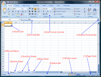
Working with workbook and worksheet

Information in Excel is stored in a Workbook. The first new workbook opened in a session is called Book1. A workbook is a collection of individual Worksheets. Each worksheet has a name that appears in a Worksheet Tab at the bottom of the workbook window. By default, these names appear as Sheet1, Sheet2, Sheet3, etc. You can change the default names, if desired

Entering data (text,Number) 

You have several options when you want to enter data manually in Excel. You can enter data in one cell, in several cells at the same time, or on more than one worksheet at once. The data that you enter can be numbers, text, dates, or times. You can format the data in a variety of ways. And, there are several settings that you can adjust to make data entry easier for you. 

Formatting (Font,number) and customizing data

Cell formatting The icons on the Home ribbon provide you with  a variety of formatting options. To apply any of these, just select the cell or cells that you want to format, and then click the desired icon.  Commonly used formatting attributes include: Font and size Bold, Italic, Underline Cell borders Background and Font color Alignment: Left, Centre or Right Merge text across multiple cells Wrap text within a cell Rotate angle of text Format number as Currency, Percentage or Decimal Increase or Decrease number of decimal places The Format Painter allows you to copy formatting attributes from one cell to a range of cells.

 

 

Editing spreadsheets

 

 Formulas and function

Creating / copying formulas 

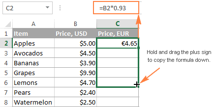
Microsoft Excel provide a really quick way to copy a formula down a column. You just do the following:

• Enter a formula in the top cell.
• Select the cell with the formula, and hover the mouse cursor over a small square at the lower right-hand corner of the cell, which is called the Fill handle. As you do this, the cursor will change to a thick black cross.
• Hold and drag the fill handle down the column over the cells where you want to copy the formula.

Cell referencing

Excel is dynamic when it comes to cell addresses. If you have a cell with a formula that references a different cell’s address and you copy the formula from the first cell to another cell, Excel updates the cell reference inside the formula. Try an example:

1.      In cell B2, enter 100.

2.      In cell C2, enter =B2*2.

3.      Press Enter.

4.      Cell C2 now returns the value 200.

5.      If C2 is not the active cell, click it once.

6.      Press Ctrl+C, or click the Copy button on the Home tab.

7.      Click cell C3.

8.      Press Ctrl+V, or click the Paste button on the Home tab.

Using insert function button

1Select the cell into which you want to enter the formula.

2. Select the Insert Function button in the Formula Bar

3Enter a description of what you want to do and press [Return].

4. Select the desired function in the Select a function list.

5. Select OK.

6. Click the Collapse Dialog button at the right of the first argument edit box.

7. Select the range you want to use in the calculation.

8. Release the mouse button.

9. Click the Expand Dialog button.

10. Repeat steps 6 to 9 for any additional arguments you need to select.

10. Select  OK

 

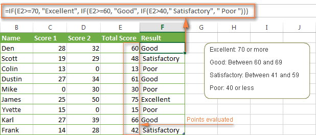
Using nested functions

A nested function uses a function as one of the arguments. Excel allows you to nest up to 64 levels of functions. Users typically create nested functions as part of a conditional formula. For example, IF(AVERAGE(B2:B10)>100,SUM(C2:G10),0). The AVERAGE and SUM functions are nested within the IF function. The structure of the IF function is IF(condition test, if true, if false). You can use the AND, OR, NOT, and IF functions to create conditional formulas. When you create a nested formula, it can be difficult to understand how Excel performs the calculations. You can use the Evaluate Formula dialog box to help you evaluate parts of a nested formula one step at a time.

 

Using SUM/COUNT/MIN/AVERAGE/RANK

example of sum 

 

example of count 

 

example of min

 

example of average

 

example of rank

 

IF statement and nested IF
 
Working with chart

Select cells A3 to D6. You must select all the cells containing the data you want in your chart. You should also include the data labels.

Choose the Insert tab.

Click the Column button in the Charts group. A list of column chart sub-types types appears.

Click the Clustered Column chart sub-type. Excel creates a Clustered Column chart and the Chart Tools context tabs appear.

Sourting and querying data

This example teaches you how to import data from a Microsoft Access database by using the Microsoft Query Wizard. With Microsoft Query, you can select the columns of data that you want and import only that data into Excel.

. On the Data tab, click From Other Sources, From Microsoft Query.

The 'Choose Data Source" dialog box appears.
2. Select MS Access Database* and check 'Use the Query Wizard to create/edit queries'.

3. Click OK.
4. Select the database and click OK.

This Access database consists of multiple tables. You can select the table and columns you want to include in your query.
5. Select Customers and click the > symbol.

6. Click Next.
To only import a specified set of records, filter the data.

7. Click City from the 'Column to filter' list and only include rows where City equals New York.

8. Click Next.
You can sort your data if you want (we don't do it here).
9. Click Next.

10. Click Finish to return the data to Microsoft Excel.

11. Select how you want to view this data, where you want to put it, and click OK.

Result:

Note: when your Access data changes, you can click Refresh to update the data in Excel.

Freeze pane
 Select the View tab from the toolbar at the top of the screen and click on the Freeze Panes button in the Window group. Then click on the Freeze Top Row option in the popup menu.
 
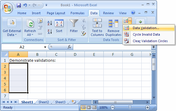
Data validation
MS Excel data validation feature allows you to set up certain rules that dictate what can be entered into a cell. For example, you may want to limit data entry in a particular cell to whole numbers between 0 and 10. If the user makes an invalid entry, you can display a custom message as shown below.

 
Linking worksheets

1. In the source worksheet, select the cell you want to link to and click the Copy button on the Home tab. Or press Ctrl+C, or right-click and select Copy.
2. Switch to the destination spreadsheet and click the cell where you want the link. Then, depending on your version of Excel:
   • Excel 2007, 2010, and 2013: On the Home tab, click the down arrow below Paste and click Paste Link. In newer versions you may also right-click and select the Paste Link from the Paste menu.
   • Excel 2003 and older versions: On the Edit menu, click Paste Special, and then click Paste Link.
3. Return to the source worksheet and press ESC to remove the animated border around the cell

Importing and Exporting data

export to word 

The simplest way to display Excel data in a Word document is to use Copy/Paste.

1. Open the destination Word document.
2. In the source Excel spreadsheet, select the data you want to copy then hit CTRL-C.
3. In the destination Word document, place the cursor where you want the data, then hit CTRL-V.

 

4. The default paste will use the Keep Source Formatting (A) paste option. This preserves any formatting you have done in Excel and pastes the data into Word as a table using that same formatting. As you can see, you may need to clean up your table after the paste to make it look correct in the new document.
5. To change the paste option, click the Ctrl dropdown option in the bottom right corner of your new table after pasting and select a new option. Other Paste options include: Use Destination Styles (B) – This will paste the data into Word as a table and adapt the display elements into the same formatting as the Word document. Use this to make your fonts and colors consistent in the destination without having to edit in Excel beforehand.

 

Copy as Picture (C) – This will paste the data range as a Word image object. You will be able to resize and edit the image as you would any other picture, but you will not be able to edit the data. The paste will use the original Excel formatting to generate the picture.

Import a word table

Open a new or existing document in Microsoft Word.

Click the "Insert" tab > Locate the "Tables" group. 

Select the "Table" icon > Choose the "Insert Table..." option.

Set the "Number of columns," "Number of rows," and "AutoFit behavior" to your desired specifications > Click [OK].

Open the Excel file and use your mouse to select the data you wish to import. 

Right-click on the range of cells you have highlighted and select "Copy."

Switch back to Word and highlight the table cells where you want to import the Excel data.

Right-click on the Word table and click the option you want under "Paste Options." 

Import a text file

There are two ways to import data from a text file by using Microsoft Excel: You can open the text file in Excel, or you can import the text file as an external data range. To export data from Excel to a text file, use the Save As command.
There are two commonly used text file formats:

• Delimited text files (.txt), in which the TAB character (ASCII character code 009) typically separates each field of text.
  
• Comma separated values text files (.csv), in which the comma character (,) typically separates each field of text.
  

You can change the separator character that is used in both delimited and .csv text files. This may be necessary to make sure that the import or export operation works the way that you want it to.
Notes  

• You can import or export up to 1,048,576 rows and 16,384 columns.